Transformers - Intuitively and Exhaustively Explained

Exploring the modern wave of machine learning: taking apart the transformer step by step

Image by Daniel Warfield using MidJourney. All images are by Daniel Warfield unless otherwise specified.

In this post you will learn about the transformer architecture, which is at the core of nearly all cutting-edge large language models. We’ll start with a brief chronology of some relevant natural language processing concepts, then we’ll go through the transformer step by step and uncover how it works.

Who is this useful for? Anyone interested in natural language processing (NLP).

How advanced is this post? This is not a complex post, but there are a lot of concepts, so it might be daunting to less experienced data scientists.

Pre-requisites: A good working understanding of a standard neural network. Some cursory experience with embeddings, encoders, and decoders would probably also be helpful.

A Brief Chronology of NLP Up to the Transformer

The following sections contain useful concepts and technologies to know before getting into transformers. Feel free to skip ahead if you feel confident.

Word Vector Embeddings

A conceptual understanding of word vector embeddings is pretty much fundamental to understanding natural language processing. In essence, a word vector embedding takes individual words and translates them into a vector which somehow represents its meaning.

The job of a word to vector embedder: turn words into numbers which somehow capture their general meaning.

The details can vary from implementation to implementation, but the end result can be thought of as a “space of words”, where the space obeys certain convenient relationships. Words are hard to do math on, but vectors which contain information about a word, and how they relate to other words, are significantly easier to do math on. This task of converting words to vectors is often referred to as an “embedding”.

Word2Vect, a landmark paper in the natural language processing space, sought to create an embedding which obeyed certain useful characteristics. Essentially, they wanted to be able to do algebra with words, and created an embedding to facilitate that. With Word2Vect, you could embed the word “king”, subtract the embedding for “man”, add the embedding for “woman”, and you would get a vector who’s nearest neighbor was the embedding for “queen”.

A conceptual demonstration of doing algebra on word embeddings. If you think of each of the points as a vector from the origin, if you subtracted the vector for “man” from the vector for “king”, and added the vector for “woman”, the resultant vector would be near the word queen. In actuality these embedding spaces are of much higher dimensions, and the measurement for “closeness” can be a bit less intuitive (like cosine similarity), but the intuition remains the same.

As the state of the art has progressed, word embeddings have remained an important tool, with GloVe, Word2Vec, FastText, and learned embeddings being popular choices. Sub-word embeddings are generally much more powerful than full word embeddings, but are out of scope of this post.

Recurrent Networks (RNNs)

Now that we can convert words into numbers which hold some meaning, we can start analyzing sequences of words. One of the early strategies was using a recurrent neural network, where you would train a neural network that would feed into itself over sequential inputs.

The general idea of an RNN, which is a normal fully connected neural network which feeds into itself.

What an RNN might look like if it had 3 hidden neurons and was used across 2 inputs. The arrows in red are the recursive connections which connect the information from subsequent recurrent layers. The blue arrows are internal connections, like a dense layer. The neural network is copied for illustrative purposes, but keep in mind the network is actually feeding back into itself, meaning the parameters for the second (and subsequent) modules would be the same as the first.

Because recurrent networks feed into themselves, they can be used for sequences of arbitrary length. They will have the same number of parameters for a sequence of length 10 or a sequence of length 100 because they reuse the same parameters for each recursive connection.

This network style was employed across numerous modeling problems which could generally be categorized as sequence to sequence modeling, sequence to vector modeling, vector to sequence modeling, and sequence to vector to sequence modeling.

Conceptual diagrams of a few applications of different modeling strategies which might use RNNs. Sequence to Sequence might be predicting the next word for text complete. Sequence to vector might be scoring how satisfied a customer was with a review. Vector to sequence might be compressing an image into a vector and asking the model to describe that image as a sequence of text. Sequence to vector to sequence might be text translation, where you need to understand a sentence, compress it into some representation, then construct a translation of that compressed representation in a different language.

While the promise of infinite length sequence modeling is enticing, it’s not practical. Because each layer shares the same weights it’s easy for recurrent models to forget the content of inputs. As a result, RNNs could only practically be used for very short sequences of words.

There were some attempts to solve this problem by using “gated” and “leaky” RNNs. The most famous of these was the LSTM, which is described in the next section.

Long/Short Term Memory (LSTMs)

The LSTM was created as an attempt to improve the ability of recurrent networks to recall important information. LSTM’s have a short term and long-term memory, where certain information can be checked into or removed from the long-term memory at any given element in the sequence.

an LSTM in a nutshell

Conceptually, an LSTM has three key subcomponents, the “forget gate” which is used to forget previous long-term memories, the “input gate” which is used to commit things to long-term memory, and the “output gate” which is used to formulate the short-term memory for the next iteration.

The parameters in an LSTM. This particular LSTM expects an input vector of dimension 3, and holds internal state vectors of dimension 2. the dimension of vectors is a configurable hyperparameter. Also, notice the “S” and “T” at the end of each of the gates. These stand for sigmoid or tanh activation functions, which are used to squash values into certain ranges, like 0 to 1 or -1 to 1. This “squashing” is what allows the network to “forget” and “commit to memory” certain information. image by the author, heavily inspired by Source

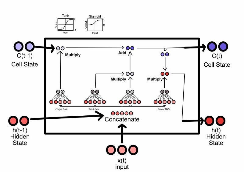
LSTMs, and similar architectures like GRUs, proved to be a significant improvement on the classic RNN discussed in the previous section. The ability to hold memory as a separate concept which is checked in and checked out of proved to be incredibly powerful. However, while LSTMs could model longer sequences, they were too forgetful for many language modeling tasks. Also, because they relied on previous inputs (like RNNs), their training was difficult to parallelize and, as a result, slow.

Attention Through Alignment

The Landmark Paper, Neural Machine Translation by Jointly Learning to Align and Translate popularized the general concept of attention and was the conceptual precursor to the multi-headed self-attention mechanisms used in transformers.

I have a whole article on this specific topic, along with example code in PyTorch. In a nutshell, the attention mechanism in this paper looks at all potential inputs and decides which one to present to an RNN at any given output. In other words, it decides which inputs are currently relevant, and which inputs are not currently relevant.

Attention from Alignment, Practically Explained

This approach proved to have a massive impact, particularly in translation tasks. It allowed recurrent networks to figure out which information is currently relevant, thus allowing previously unprecedented performance in translation tasks specifically.

A figure from my article on Attention. The squares represent the word vector embeddings, and the circles represent intermediary vector representations. The red and blue circles are hidden states from a recurrent network, and the white circles are hidden states created by the attention through alignment mechanism. The punchline is that the attention mechanism can choose the right inputs to present to the output at any given step.

The Transformer

In the previous sections we covered some forest through the trees knowledge. Now we’ll look at the transformer, which used a combination of previously successful and novel ideas to revolutionize natural language processing.

The transformer diagram. Source

We’ll go through the transformer element by element and discuss how each module works. There’s a lot to go over, but it’s not math-heavy and the concepts are pretty approachable.

High Level Architecture

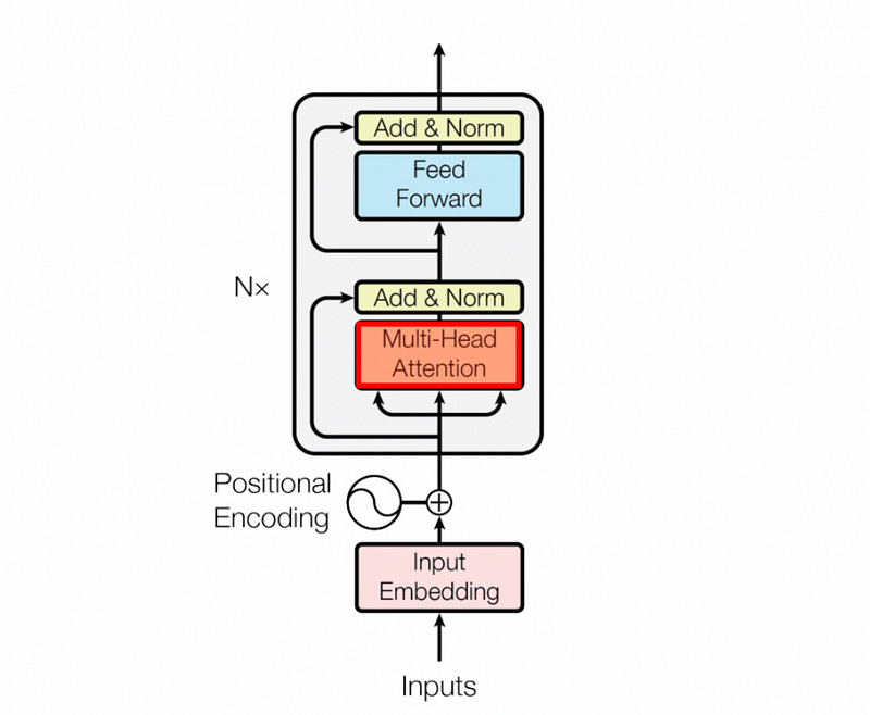
At its most fundamental, the transformer is an encoder/decoder style model, kind of like the sequence to vector to sequence model we discussed previously. The encoder takes some input and compresses it to a representation which encodes the meaning of the entire input. The decoder then takes that embedding and constructs the output.

A transformer working in a sequence to vector to sequence task, in a nutshell. The input (I am a manager) is compressed to some abstract representation that encodes the meaning of the entire input. The decoder works to construct the output.

Input Embedding and Positional Encoding

The input embedding for a transformer is similar to previously discussed strategies; a word space embedder similar to word2vect converts all input words into a vector. This embedding is trained alongside the model itself, as essentially a lookup table which is improved through model training. So, there would be a randomly initialized vector corresponding to each word in the vocabulary, and this vector would change as the model learned about each word.

Unlike recurrent strategies, transformers encode the entire input in one shot. As a result the encoder might lose information about the location of words in an input. To resolve this, transformers also use positional encoders, which is a vector encoding information about where a particular word was in the sequence.

"""
Plotting positional encoding for each index.
A positional encoding for a single token would be a horizontal row in the image

inspired by https://machinelearningmastery.com/a-gentle-introduction-to-positional-encoding-in-transformer-models-part-1/
"""

import numpy as np
import matplotlib.pyplot as plt

#these would be defined based on the vector embedding and sequence
sequence_length = 512
embedding_dimension = 1000

#generating a positional encodings
def gen_positional_encodings(sequence_length, embedding_dimension):
    #creating an empty placeholder
    positional_encodings = np.zeros((sequence_length, embedding_dimension))

    #itterating over each element in the sequence
    for i in range(sequence_length):

        #calculating the values of this sequences position vector
        #as defined in section 3.5 of the attention is all you need
        #paper: https://arxiv.org/pdf/1706.03762.pdf
        for j in np.arange(int(embedding_dimension/2)):
            denominator = np.power(sequence_length, 2*j/embedding_dimension)
            positional_encodings[i, 2*j] = np.sin(i/denominator)
            positional_encodings[i, 2*j+1] = np.cos(i/denominator)

    return positional_encodings

#rendering
fig, ax = plt.subplots(figsize=(15,5))
ax.set_ylabel('Sequence Index')
ax.set_xlabel('Positional Encoding')
cax = ax.matshow(gen_positional_encodings(sequence_length, embedding_dimension))
fig.colorbar(cax, pad=0.01)

Example of positional encoding. The Y axis represents subsequent words, and the x axis represents values within a particular words positional encoding. Each row in this image represents an individual word.

"""
Rendering out a few individual examples

inspired by https://machinelearningmastery.com/a-gentle-introduction-to-positional-encoding-in-transformer-models-part-1/
"""
positional_encodings = gen_positional_encodings(100, 50)
fig = plt.figure(figsize=(15, 4))    
for i in range(4):
    ax = plt.subplot(141 + i)
    idx = i*10
    plt.plot(positional_encodings[:,idx])
    ax.set_title(f'positional encoding {idx}')
plt.show()

Values of the position vector relative to different indexes in a sequence. K represents the index in a sequence, and the graph represents values in a vector.

This system uses the sin and cosin function in unison to encode position, which you can gain some intuition about in this article:

Use Frequency More Frequently

I won’t harp on it, but a fascinating note; this system of encoding position is remarkably similar to positional encoders used in motors, where two sin waves offset by 90 degrees allow a motor driver to understand position, direction, and speed of a motor.

The vector used to encode the position of a word is added to the embedding of that word, creating a vector which contains both information about where that word is in a sentence, and the word itself. You might think “if your adding these wiggly waves to the embedding vector, wouldn’t that mask some of the meaning of the original embedding, and maybe confuse the model”? To that, I would say that neural networks (which the transformer employs for it’s learnable parameters) are incredibly good at understanding and manipulating smooth and continuous functions, so this is practically of little consequence for a sufficiently large model.

Multi-Headed Self Attention: High Level

This is probably the most important sub-component of the transformer mechanism.

The multi-headed self-attention mechanism within the original diagram. Source

In this author’s humble opinion, calling this an “attention” mechanism is a bit of a misnomer in a linguistic sense. Really, it’s a “co-relation” and “contextualization” mechanism. It allows words to interact with other words to transform the input (which is a list of embedded vectors for each word) into a matrix which represents the meaning of the entire input.

Multi Headed self-attention, in a nutshell. The mechanism mathematically combines the vectors for different words, creating a matrix which encodes a deeper meaning of the entire input.

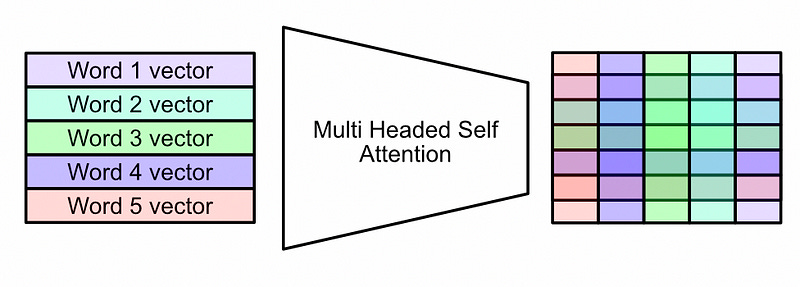
This mechanism can be thought of as four individual steps:

1. Creation of the Query, Key, and Value

2. Division into Multiple Heads

3. The Attention Head

4. Composing the Final Output

Multi Head Self Att. Step 1): Creation of the Query, Key, and Value

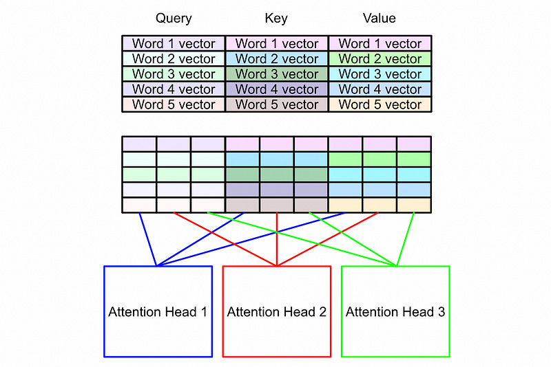
First of all, don’t be too worried about the names “Query”, “Key”, and “Value”. These are vaguely inspired by databases, but really only in the most obtuse sense. The query, key, and value are essentially different representations of the embedded input which will be co-related to each-other throughout the attention mechanism.

Turning the embedded input into the query key and value. The input has a dimension which is num_words by embedding_size, The query, key, and value all have the same dimensions as the input. In essence, a dense network projects the input into a tensor with three times the number of features while maintaining sequence length.

The dense network shown above includes the only learnable parameters in the multi headed self-attention mechanism. Multi headed self-attention can be thought of as a function, and the model learns the inputs (Query, Key, and Value) which maximizes the performance of that function for the final modeling task.

Multi Head Self Att. Step 2): Division into multiple heads

Before we do the actual contextualization, which makes self-attention so powerful, we’re going to divide the query, key, and value into chunks. The core idea is that instead of co-relating our words one way, we can co-relate our words numerous different ways. In doing so we can encode more subtle and complex meaning.

In this example we have 3 attention heads. As a result the query, key, and value are divided into 3 sections and passed to each head. Note that we’re dividing along the feature axis, not the word axis. Different aspects of each word’s embedding are passed to a different attention head, but each word is still present for each attention head.

Multi Head Self Att. Step 3): The Attention Head

Now that we have the sub-components of the query, key, and value which is passed to an attention head, we can discuss how the attention head combines values in order to contextualize results. In Attention is all you need, this is done with matrix multiplication.

Matrix Multiplication. Source

In matrix multiplication rows in one matrix get combined with columns in another matrix via a dot product to create a resultant matrix. In the attention mechanism the Query and Key are matrix multiplied together to create what is sometimes referred to as the “z” matrix.

Calculating the “z matrix” with the query and key. Note that the key is transposed to allow for matrix multiplication to result in the correct attention matrix shape.

This is a fairly simple operation, and as a result it’s easy to underestimate its impact. The usage of a matrix multiplication at this point forces the representations of each word to be combined with the representations of each other word. Because the Query and Key are defined by a dense network, the neural network learns how to translate the query and key to optimize the content of this matrix.

After the “z” matrix is calculated, an operation called “softmax” is performed across rows. Softmax is the process of taking a list of numbers and turning them into a list of probabilities. Big numbers in the list become big probabilities, and small numbers become small probabilities. Because the “z” matrix is a relation of every word with every other word, softmaxing turns the z matrix into a matrix of probabilities that this word should interact with another word. This is very similar to the idea of attention we discussed previously, accept instead of trying to define which input words relate with which output words, self-attention tries to define which input words should interact with other input words to create a more context rich understanding of the input.

Now that we have the attention matrix, it can be multiplied by the value matrix. The attention matrix specifies which words should interact with other words, and the value matrix contains the representations of the words.

The attention matrix multiplied by the value matrix to yield the final result of the attention mechanism. Because of the shape of the attention matrix, the result is the same shape as the value matrix. Keep in mind, this is the result from a single attention head.

self-attention is the most complex concept in the transformer. If you want some additional insight, I recommend checking out my article on attention through alignment so you can build a thorough understanding of the general concept of attention

Attention from Alignment, Practically Explained

then checking out my article where I go through the math of multi-headed self-attention by hand.

Multi-Headed Self Attention — By Hand

Multi Head Self Att. Step 4): Composing the final output

In the last section we used the query, key, and value to construct a new result matrix which has the same shape as the value matrix, but with significantly more context awareness.

Recall that the attention head only computes the attention for a subcomponent of the input space (divided along the feature axis).

Recall that the inputs were split into multiple attention heads. In this example, 3 heads.

Each of these heads now outputs a different result, which can then be concatenated together.

The results of each attention head gets concatenated together.

The shape of the output matrix is the same exact shape as the input matrix. However, unlike the input where each row related cleanly with a singular word, this matrix is much more abstract.

Recall that the attention mechanism, in a nutshell, transforms the embedded input into an abstract context rich representation.

Add and Norm

Add and Norm within the original diagram. Source

The Add and Norm operations are applied twice in the encoder, and both times its effect is the same. There’s really two key concepts at play here; skip connections and layer normalization.

Skip connections are used all over the shop in machine learning. my favorite example is in image segmentation using a U-net architecture, if you’re familiar with that. Basically, when you do complex operations, it’s easy for the model to “get away from itself”. This has all sorts of fancy mathematical definitions like gradient explosions and rank collapse, but conceptually it’s pretty simple; a model can overthink a problem, and as a result it can be useful to re-introduce older data to re-introduce some of that simpler structure.

What a skip connected add might look like. In this example the matrix on the left represents the original encoded input. The matrix in the middle represents the hyper contextual result from the attention matrix. The Right represents the result of a skip connection: a context aware matrix which still contains some order from the original input.

Layer normalization is similar to skip connections in that it, conceptually, reigns in wonkiness. A lot of operations have been done to this data, which has resulted in who knows how large and small of values. If you do data science on this matrix, you might have to deal with both incredibly small and massively large values. This is known to be problematic.

Layer normalization computes the mean and standard deviation (how widely distributed the values are) and uses those values to squash the data back into a reasonable distribution.

Feed Forward

Feed Forward within the original diagram. Source

This part’s simple. We can take the output from the add norm after the attention mechanism and pass it through a simple dense network. The output of the feed forward network is then passed through another add norm layer, and that results in the final output. This final output will be used by the decoder.

General Function of the Decoder

We’ve completely covered the encoder and now have a highly contextualized representation of the input. Now we’ll discuss how the decoder uses that representation to generate some output.

High level representation of how the output of the encoder relates to the decoder. the decoder references the encoded input for every recursive loop of the output.

The decoder is very similar to the encoder with a few minor variations. Before we talk about the variations, let's talk about similarities

The Transformer Architecture. Source

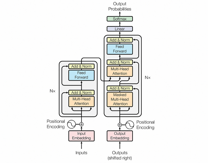
As can be seen in the image above, the decoder uses the same word to vector embedding approach, and employs the same positional encoder. The decoder uses “Masked” multi headed self attention, which we’ll discuss in the next section, and uses another multi-headed attention block.

The second multi-headed self attention in the decoder uses the encoded input for the key and value, and uses the decoder input to generate the query. As a result, the attention matrix gets calculated from the embedding for the encoder and the decoder, which then gets applied to the value from the encoder. This allows the decoder to decide what it should finally output based on both the encoder input and the decoder input.

The rest is the same boiler plate you might find on any other model. The results pass through another feed forward, an add norm, a linear layer, and a softmax. This softmax would then output probabilities for a bag of words, for instance, allowing the model to decide on a word to output.

Masked Multi Headed Self Attention

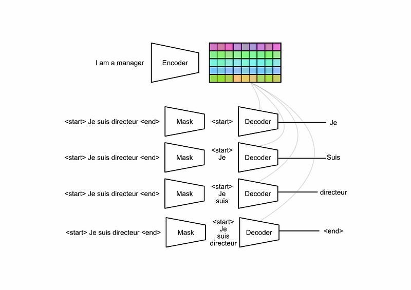
So the only thing really new about the decoder is the “masked” attention. This has to do with how these models are trained.

One of the core flaws of recurrent neural networks is that you need to train them sequentially. An RNN intimately relies on the analysis of the previous step to inform the next step.

RNNs intimate dependencies between steps.

This makes training RNNs incredibly slow as each sequence in the training set needs to be sequentially fed through the model one by one. With some careful modifications to the attention mechanism transformers can get around this problem, allowing the model to be trained for an entire sequence in parallel.

The details can get a bit fiddly, but the essence is this: When training a model, you have access to the desired output sequence. As a result, you can feed the entire output sequence to the decoder (including outputs you haven’t predicted yet) and use a mask to hide them from the model. This allows you to train on all positions of the sequence simultaneously.

A diagram of the mask working in mask multiheaded self-attention, for an English to French translation task. The input of this task is the phrase “I am a manager” and the desired output is the phrase “Je suis directeur”. Note, for simplicities sake, I’ve generally neglected the concept of utility tokens. They’re pretty easy to understand, though: start the sequence, end the sequence, etc.

Conclusion

And that’s it! We broke down some of the technical innovations that lead to the discovery of the transformer and how the transformer works, then we went over the transformer’s high-level architecture as an encoder-decoder model and discussed important sub-components like multi-headed self-attention, input embeddings, positional encoding, skip connections, and normalization.

---

This post was brought to you by Daniel Warfield, author of the Intuitively And Exhaustively Explained Series (IAEE). IAEE dives into the fundamentals of LLMs with engaging and detailed explanations on the technology that shapes current language models.